DATA MINING Desktop Survival Guide by Graham Williams
Desktop Survival Project Home Introduction Getting Started The Business Problem Data Loading Data Exploring Data Interactive Graphics Statistical Tests Models Network Analysis Text Mining Decision Trees Random Forests Boosting Bagging Support Vector Machine Linear Regression Neural Network Naive Bayes Survival Analysis Evaluation and Deployment Transforming Data Deployment Troubleshooting Issues Moving into R R Getting Help Data Graphics in R Understanding Data Preparing Data Issues Evaluating Models Reporting Fraud Analysis Archetype Analysis Algorithms Bayes Classifier K-Nearest Neighbours Linear Models Open Products AlphaMiner Borgelt Data Mining Suite KNime R Rattle Weka Closed Products Clementine Equbits Foresight GhostMiner InductionEngine ODM Enterprise Miner Statistica Data Miner TreeNet Virtual Predict Installing Rattle Projects Bibliography Index Preface Goals Organisation Features Audience Typographical Conventions A Note on Languages Currency Acknowledgements Introduction Data Mining The Business Problem Types of Analysis Data Mining Applications A Framework for Modelling Agile Data Mining R Rattle Why R and Rattle? Data Preparation Number of Algorithms Repeatability Performance Open Source Data Mining Business Case Sample Business Case Pros and Cons Books on R Getting Started Initial Interaction with R Quitting Rattle and R First Contact Loading a Dataset Building a Model Understanding Our Data Evaluating the Model Evaluating the Model Interacting with R Interacting with Rattle Projects Toolbar Menus Interacting with Plots Keyboard Navigation Summary Command Summary The Business Problem Solar Panel Efficiency Water Collection Others Other Business Problems Fraud Detection Loan Approval Documenting the Business Problem Summary Resources Exercises Data Data Nomenclature Loading Data into Rattle CSV Data Datasets Reading Direct from URL Play Golf Weather Data Other Data Sources ARFF Data ODBC Sourced Data Setting Up a Data Source Name Netezza Setup Teradata Setup R Data R Dataset Data Entry Data Tab Options in Rattle Sampling Data Variable Roles Automatic Role Identification Weights Calculator Manipulating Data Loading Data CSV Data Locating and Loading Data Loading the File CSV Options Basic Data Summary ARFF Data ODBC Sourced Data R Dataset R Data Library Data Options Sampling Data Variable Roles Automatic Role Identification Weights Calculator Command Summary Exploring Data Summarising Data Summary Describe Basics Kurtosis Skewness Missing Exploring Distributions Box Plot Histogram Cumulative Distribution Plot Benford's Law Other Digits Stratified Benford Plots Bar Plot Dot Plot Mosaic Plot GGobi Scatterplot Data Viewer Brushing Identify Multivariate Outliers Other Options Quality Plots Using R Further GGobi Documentation Correlation Analysis Hierarchical Correlation Principal Components Single Variable Overviews Interactive Graphics Interactive Visualisations Latticist GGobi Scatterplot Multiple Plots Brushing Other Plots Data Viewer Brushing Identify Multivariate Outliers Other Options Quality Plots Using R Further GGobi Documentation Documenting Interactive Explorations Code Review Chapter Exercises Command Summary Statistical Tests Documenting Interactive Explorations Code Review Further Resources Chapter Exercises Command Summary Models A Framework for Modelling Descriptive Analytics Predictive Analytics Documenting Models Summary Code Review Exercises Further Resources Command Summary Cluster Analysis Summary Clusters Basic Clustering Hot Spots Alternative Clustering Other Cluster Examples KMeans Export KMeans Clusters Discriminant Coordinates Plot Number of Clusters Hierarchical Clusters Other Cluster Algorithms Association Analysis Summary Overview Algorithm Usage Read Transactions file format sep cols rm.duplicates Summary Apriori data parameter appearance control Inspect Examples Video Marketing Survey Data Other Examples Resources and Further Reading Basket Analysis General Rules Network Analysis Documenting Interactive Explorations Code Review Chapter Exercises Command Summary Text Mining Application to Text Text Mining with R Decision Trees Knowledge Representation Search Heuristic Measures Tutorial Example Rattle R Tuning Parameters Min Split (Rarg[]minsplit) Min Bucket (minbucket) Priors (prior) Loss Matrix Complexity (cp) Other Options Simple Example Convert Tree to Rules Predicting Salary Group Issues Summary Code Review Iris Wine Exercises Resources Command Summary Random Forests Formalities Tutorial Example Tuning Parameters Number of Trees Sample Size Number of Variables Summary Overview Algorithm Usage Random Forest importance classwt Examples Resources and Further Reading Summary Overview Example Algorithm Resources and Further Reading Boosting Formalities Tutorial Example Tuning Parameters Summary Overview AdaBoost Algorithm Examples Step by Step Using gbm Extensions and Variations Alternating Decision Tree Resources and Further Reading Documenting Code Review Further Resources Chapter Exercises Command Summary Bootstrapping Summary Usage Further Information Summary Overview Example Algorithm Resources and Further Reading Bagging Support Vector Machine Formalities Tutorial Example Tuning parameters Examples Resources and Further Reading Overview Examples Resources and Further Reading Linear Regression Linear Regression Formalities Tutorial Example Tuning parameters Generalized Regression Formalities Tutorial Example Tuning parameters Logistic Regression Formalities Tutorial Example Tuning parameters Discussion Probit Regression Formalities Tutorial Example Tuning Parameters Multinomial Regression Formalities Tutorial Example Tuning Parameters Neural Network Formalities Tutorial Example Tuning parameters Documenting Code Review Further Resources Chapter Exercises Command Summary Naive Bayes Summary Code Review Resources Exercises Command Summary Survival Analysis Sample Data Simple Lung Descriptive Analysis Regression survreg Simple Lung coxph Simple Lung Apply to New Data More Input Variables Decision Tree Example from Singer and Willett Other Approaches Design Package Random Survival Forests Prediction on Test Data Evaluation The Evaluate Tab Confusion Matrix Measures Graphical Measures Risk Charts Cost Curves Lift ROC Curves Area Under Curve Precision versus Recall Sensitivity versus Specificity Predicted versus Observed Scoring Documenting Interactive Explorations Code Review Chapter Exercises Command Summary Transforming Data Rescale Data Recenter Scale [0,1] Rank Median/MAD Peer Relativity Profiling Index Impute Zero/Missing Mean/Median/Mode Constant Remap Binning Indicator Variables Join Categorics Math Transforms Outliers Cleanup Delete Ignored Delete Selected Delete Missing Delete Obs with Missing Other Transformations Removing Duplicates Command Summary Deployment Documenting Deployment Code Review Chapter Exercises Command Summary Troubleshooting Cairo A factor has new levels Issues Model Selection Overfitting Imbalanced Classification Sampling Cost Based Learning Model Deployment and Interoperability SQL PMML XML for Data Bibliographic Notes Documenting Code Review Chapter Exercises Command Summary Moving into R Interacting with R Basic Command Line Windows, Icons, Mouse, Pointer--WIMP The Current Rattle State Samples Projects The Rattle Log Further Tuning Models Emacs and ESS Documenting Code Review Chapter Exercises Command Summary R Evaluation Exercises Assignment Libraries and Packages Searching for Objects Package Management Information About a Package Testing Package Availability Packages and Namespaces Basic Programming in R Principles Folders and Files Flow Control If Statement For Loop Functions Apply Methods Objects System Running System Commands System Parameters Misc Internet Memory Management Memory Usage Garbage Collection Errors Frivolous Sudoku Further Resources Using R Specific Purposes Survey Analysis Getting Help R Documentation Data Data Types Numbers Strings Building Strings Splitting Strings Substitution Trim Whitespace Evaluating Strings Logical Dates and Times Space Data Structures Vectors Arrays Lists Sets Matricies Exercises Data Frames Accessing Columns Removing Columns Exercises General Manipulation Factors Elements Rows and Columns Finding Index of Elements Partitions Head and Tail Reverse a List Sorting Unique Values Loading Data Interactive Responses Interactive Data Entry Available Datasets The Iris Dataset CSV Data Used In The Book The Wine Dataset The Cardiac Arrhythmia Dataset The Adult Survey Dataset Foreign Formats Stata Data Conversions Reading Variable Width Data Saving Data Formatted Output Automatically Generate Filenames Reading a Large File Manipulating Data Manipulating Data As SQL Using SQLite ODBC Data Database Connection Excel Access Clipboard Data Spatial Data Simple Map A Density Map Overlays and Point in Polygon Other Data Formats Fixed Width Data Global Positioning System Documenting a Dataset Common Data Problems Graphics in R Basic Plot Controlling Axes Arrow Axes Legends and Points Tables Within Plots Colour Labels in Plots Axis Labels Legend Labels Within Plots Maths in Labels Multiple Plots MatPlot Multiple Plots Using ggplot2 Using GGPlot Networks Symbols Other Graphic Elements Making an Animation Animated Mandelbrot Adding a Logo to a Graphic Graphics Devices Setup Screen Devices Multiple Devices File Devices Multiple Plots Copy and Print Devices Graphics Parameters Plotting Region Locating Points on a Plot Scientific Notation and Plots Understanding Data Single Variable Overviews Textual Summaries Multiple Line Plots Separate Line Plots Pie Chart Fan Plot Stem and Leaf Plots Histogram Barplot Trellis Histogram Histogram Uneven Distribution Bump Chart Density Plot Basic Histogram Basic Histogram with Density Curve Practical Histogram Multiple Variable Overviews Scatterplot Scatterplot with Marginal Histograms Multi-Dimension Scatterplot Correlation Plot Colourful Correlations Fluctuation Plot Heat Map Projection Pursuit RADVIZ Parallel Coordinates Categoric and Numeric Measuring Data Distributions Textual Summaries Boxplot Multiple Boxplots Boxplot by Class Tuning a Boxplot Boxplot Using Lattice Boxplot Using ggplot Violin Plot What Distribution Miscellaneous Plots Line and Point Plots Matrix Data Multiple Plots Aligned Plots Probability Scale Network Plot Sunflower Plot Stairs Plot Graphing Means and Error Bars Bar Charts With Segments Bar Plot With Means 3d Bar Plot Stacks Versus Lines Multi-Line Title Mathematics Plots for Normality Basic Bar Chart Bar Chart Displays Multiple Dot Plots Alternative Multiple Dot Plots 3D Plot Clustered Box Plot Perspective Plots Star Plot Residuals Plot Waterfall Plots Dates and Times Simple Time Series Multiple Time Series Plot Time Series Plot Time Series with Axis Labels Grouping Time Series for Box Plot Time Series Heatmap Textual Summaries Stem and Leaf Plots Histogram Barplot Density Plot Basic Histogram Basic Histogram with Density Curve Practical Histogram Correlation Plot Colourful Correlations Measuring Data Distributions Textual Summaries Boxplot Multiple Boxplots Boxplot by Class Box and Whisker Plot Box and Whisker Plot Clustered Box Plot Further Resources Map Displays Further Resources Preparing Data Data Selection and Extraction Training and Test Datasets Data Cleaning Review Data Selectively Changing Vector Values Replace Indices By Names Missing Values Remove Levels from a Factor Variable Manipulations Remove Columns Reorder Columns Remove Non-Numeric Columns Remove Variables with no Variance Cleaning the Wine Dataset Cleaning the Cardiac Dataset Cleaning the Survey Dataset Imputation Nearest Neighbours Multiple Imputation Data Linking Simple Linking Record Linkage Data Transformation Aggregation Sum of Columns Pivot Tables Normalising Data Binning Interpolation Variable Selection Classification Classification Classification Issues Incremental or Online Modelling Model Tuning Tuning rpart Unbalanced Classification Building Models Temporal Analysis Evaluation Basics Basic Measures Cross Validation Graphical Performance Measures Lift The ROC Curve Other Examples 10 Fold Cross Validation Area Under Curve Calibration Curves Reporting Generating Open Document Format Getting Started with odfWeave OpenOffice.org Macro Support Generating HTML Generating PDF with LATEX Configuration Figure Sizes Fraud Analysis Archetype Analysis

CSV Data

One of the simplest and most common ways of sharing data today is via the CSV format. The Spreadsheet option of the Data tab provides an easy way to load data from many different sources into Rattle.

CSV is an abbreviation of ``comma separated value'' and is a standard file format often used to exchange data between applications. CSV files can be exported from spreadsheets and databases, including OpenOffice Calc, Gnumeric, MS/Excel, SAS/Enterprise Miner, Teradata and Netezza Data Warehouses, and many, many, other applications.

This is a pretty good option for importing our data into Rattle, although it does lose meta data information (that is, information about the data types of the dataset). Without this meta data R sometimes guesses at the wrong data type for a particular column, but it isn't usually fatal!

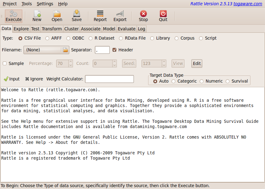
To load a dataset from a CSV file, click in the Filename button (Figure 4.2) to display a file chooser dialogue (Figure 4.3).

Figure 4.2: The toolbar and Spreadsheet options of the Data tab of the Rattle window. Click the Filename button to browse to a CSV file anywhere on your system.

Figure 4.3: The CSV file chooser showing just those files with a .csv extension in the folder. We can also select to display just the .txt files (e.g., the extension often used for tab delimited files) or else all files by selecting from the drop down menu at the bottom right.

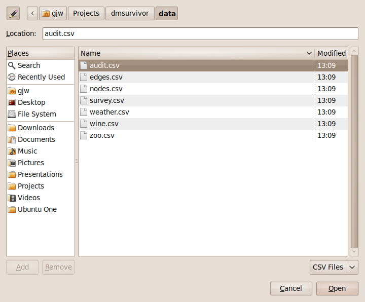We use the CSV file chooser dialogue to browse our file system to find the file we wish to load into Rattle. By default, only files that have a .csv extension will be listed (together with folders).

The pull down menu near the bottom right of the file chooser dialogue (above the Open button) allows us to select alternative filters for the files listed. We can list files that end with a .csv or a .txt, or else we can list all files.

The panel within the left region of the popup allows us to browse to the different file systems available to us, while the series of buttons along the top allow us to navigate through a series of folders on a single file system. Once we have navigated to the folder containing the CSV file we wish to load we can select this file in the main panel of the file chooser dialogue. Clicking the Open button tells Rattle that this is the file we are interested in (without yet actually loading it).

So we have not yet told Rattle to actually load the data--we have just identified where the data is. We now click the Execute button (or press the F5 key) to load the dataset from the file on the hard disk into the computer's memory, for processing by Rattle.

A sample CSV file is provided by Rattle and is called weather.csv. It will have been installed when Rattle was installed and we can find it's actual location with the system.file function which we type into the R Console:

> system.file("csv", "weather.csv", package = "rattle")

[1] "/usr/local/lib/R/site-library/rattle/csv/weather.csv"

The location reported by this function will depend on your installation. Here we see the location as it might be on a GNU/Linux system.

We can review the contents of the file using the file.show function:

> file.show(system.file("csv", "weather.csv", 
                        package = "rattle"))

As we saw in Chapter  the simplest way to load this file into Rattle is to leave the Spreadsheet option's Filename entry empty and click the Execute button. You will be asked whether you would like to load the weather dataset--choose Yes.

The top of the weather.csv file will be similar to the following (perhaps with quotes around values, although they are not necessary, and perhaps with some different values, and for brevity the header row is skipped):

2007-11-01,Canberra,8,24.3,0,3.4,6.3,NW,30,SW,NW,6,20,68,29,1019.7...
2007-11-02,Canberra,14,26.9,3.6,4.4,9.7,ENE,39,E,W,4,17,80,36,1012.4...
2007-11-03,Canberra,13.7,23.4,3.6,5.8,3.3,NW,85,N,NNE,6,6,82,69,1009.5...
2007-11-04,Canberra,13.3,15.5,39.8,7.2,9.1,NW,54,WNW,W,30,24,62,56,1005.5...
2007-11-05,Canberra,7.6,16.1,2.8,5.6,10.6,SSE,50,SSE,ESE,20,28,68,49,1018.3...
2007-11-06,Canberra,6.2,16.9,0,5.8,8.2,SE,44,SE,E,20,24,70,57,1023.8...
2007-11-07,Canberra,6.1,18.2,0.2,4.2,8.4,SE,43,SE,ESE,19,26,63,47,1024.6...

As we can see, a CSV file is actually a normal text file that we could load into any text editor to review its contents. A CSV file usually begins with a header row, listing the names of the variables, each separated by a comma. If any name (or indeed, any value in the file) contains an embedded comma, then that name (or value) will be surrounded by quote marks. The remainder of the file after the header is expected to consist of rows of data that record information about the observations, with fields separated by commas recording the values of the variables for this observation.

As we noted above, after identifying the file to load we now need to click the Execute button to actually load the dataset into Rattle. The main text panel of the Data tab changes to list the variables, together with their types and roles, and some other useful information (Figure ).

Loading data into Rattle from a CSV file simply uses the R function read.csv. We can see this to be the case by reviewing the contents of the Log tab. The function is simply used as follows:

> crs$dataset <- read.csv("file:.../weather.csv", 
                          na.strings=c(".", "NA", "", "?"))

Here, the full path to the file is left out for brevity. There are two things to note here. The first is that the dataset is loaded into a variable called crs$dataset. This is an internal variable used by Rattle. In fact, it is an element of a list variable called crs (current rattle state) and the element itself is called dataset.

The second thing to note is that by default Rattle will treat any one of four strings as representing missing values (NAs in R). This captures the most common approaches to representing missing values. SAS, for example, uses the dot (``.'') to denote missing values and R uses the special string ``NA'' to denote missing values. Other applications imply leave use the empty string, whilst yet others (including machine learning applications like C4.5) use the question mark (``?'').

For our convenience as we work on examples through the remainder of the book, we will also load the dataset from Rattle as the weather dataset. After loading the Rattle package we can make the dataset know to R with the data function:

> data(weather)

This will be equivalent to reading the data from the CSV file.

The Rattle interface provides a number of options for tuning how we read the data from a CSV file, as we can see in Figure 4.2. We can choose the field delimiter through the Separator entry. A comma is the default. To load a .txt file which uses a tab as the field separator enter the special code \\t (that is, two slashes followed by a t) as the separator. You can also leave the separator empty and any white space will be used as the separator.

The other option of interest when loading a dataset is the Header check box. Generally, CSV files have as their first row the column names. These column names will be used with R and Rattle as the names of the variables. However, not all CSV files include headers, and if that is the case for a file we want to load into Rattle the click the check box to remove the check mark. On loading a CSV file that does not contain headers R will generate variable names.

UP TO HERE

Todo: Requires updating to the Weather data once we have the final form of the weather dataset available.

We can start getting an idea of the shape of the data from this simple summary. For example, the first two variables, ID and Age, are both identified as integers (int). The first few values of ID are 1004641, 1010229, 1024587, and so on. They all appear to be of the same length (i.e, the same number of digits) and together with having a name like ID provides a very strong indicator that this is some kind of identifier for each observation. The first few values of Age are 38, 35, 32, 45, 60, and so on.

The next variable, Employment, illustrates how R deals with categoric variables. In R terms it is a Factor with 8 levels (i.e., 8 possible values). The levels begin with "Consultant" and "Private". The following sequence of numbers, all of which happen to be 2 for the first 10 observations of this dataset, discloses how R stores categoric data. Effectively, R maintains an integer indexed table, associating the levels with integers, so that "Consultant" is associated with 1, "Private" with 2, and so on. Then only these integers need to be stored for each observation, which is generally more efficient on memory usage. We see this more convincingly for the following categoric variables, Education, Marital, and Occupation (because they have more than just a single level displayed in this summary).

The seventh variable, Income, has been identified as a more general numeric rather than specific integer variable. The display of the first few values does not actually give us any insight as to why this might be so, but reviewing the actual CSV data as above we see that the third observation actually has a value of $154676.74$ for Income, indicating that these values are real numbers rather than just integers.

We also note that Adjusted, for example, looks like it might be a categoric variable, with values 0 and 1, but R identifies it as an integer! That's fine for our purposes here. We can always changes this later.

Support further development through the purchase of the PDF version of the book.
The PDF version is a formatted comprehensive draft book (with over 800 pages).
Brought to you by Togaware. This page generated: Sunday, 22 August 2010